Find the Relationship:
An Exercise in Graphing Analysis

In several laboratory investigations you do this year, a primary purpose will be to find the mathematical relationship between two variables. For example, you might want to know the relationship between the pressure exerted by a gas and its temperature. In another experiment, you might be asked to determine the relationship between the volume of a confined gas and the pressure it exerts. A very important method for determining mathematical relationships in laboratory science makes use of graphical methods. In this exercise, you will use LabQuest to help you determine several of these relationships.

OBJECTIVES

In this experiment, you will determine several mathematical relationships using graphical methods.

Example 1

Suppose you have these four ordered pairs, and you want to determine the relationship between x and y:

x y

2 6

3 9

5 15

9 27

The first logical step is to make a graph of y versus x.

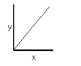
Since the shape of the plot is a straight line that passes through the origin (0,0), it is a simple direct relationship. An equation is written showing this relationship: y = k•x. This is done by writing the variable from the vertical axis (dependent variable) on the left side of the equation, and then equating it to a proportionality constant, k, multiplied by x, the independent variable. The constant, k, can be determined either by finding the slope of the graph or by solving your equation for k (k = y/x), and finding k for one of your ordered pairs. In this simple example, k = 6/2 = 3. If it is the correct proportionality constant, then you should get the same k value by dividing any of the y values by the corresponding x value. The equation can now be written:

y = 3•x (y varies directly with x)

Example 2

Consider these ordered pairs:

x y

1 2

2 8

3 18

4 32

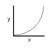
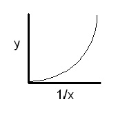
First plot y versus x. The graph looks like this:

Since this graph is not a straight line passing through the origin, you must make another graph. It appears that y increases as x increases. However, the increase is not proportional (direct). Rather, y varies exponentially with x. Thus y might vary with the square of x or the cube of x. The next logical plot would be y versus x². The graph looks like this:

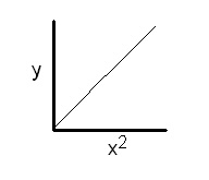
Since this plot is a straight line passing through the origin, y varies with the square of x, and the equation is:

y = k•x²

Again, place y on one side of the equation and x² on the other, multiplying x² by the proportionality constant, k. Determine k by dividing y by x²:

k = y/x² = 8/(2)² = 8/4 = 2

This value will be the same for any of the four ordered pairs, and yields the equation:

y = 2•x² (y varies directly with the square of x)

Example 3:

x y

2 24

3 16

4 12

8 6

12 4

A plot of y versus x gives a graph that looks like this:

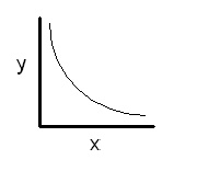
A graph with this curve always suggests an inverse relationship. To confirm an inverse relationship, plot the reciprocal of one variable versus the other variable. In this case, y is plotted versus the reciprocal of x, or 1/x. The graph looks like this:

Since this graph yields a straight line that passes through the origin (0,0), the relationship between x and y is inverse. Using the same method we used in examples 1 and 2, the equation would be:

y = k(1/x) or y = k/x

To find the constant, solve for k (k = y•x). Using any of the ordered pairs, determine k:

k = 2 X 24 = 48

Thus the equation would be:

y = 48/x (y varies inversely with x)

Example 4:

The fourth and final example has the following ordered pairs:

x y

1.0 48.00

1.5 14.20

2.0 6.00

3.0 1.78

4.0 0.75

A plot of y versus x looks like this:

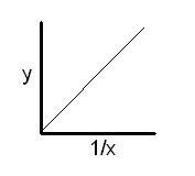
Thus the relationship must be inverse. Now plot y versus the reciprocal of x. The plot of y versus 1/x looks like this:

Since this graph is not a straight line, the relationship is not just inverse, but rather inverse square or inverse cube.

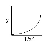
The next logical step is to plot y versus 1/x² (inverse square). The plot of this graph is shown below. The line still is not straight, so the relationship is not inverse square.

Finally, try a plot of y versus 1/x³. Aha! This plot comes out to be a straight line passing through the origin.

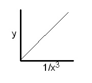
This must be the correct relationship. The equation for the relationship is:
y = k(1/x³) or y = k/x³

Next, determine a value for the constant, k. For example, k = y•x³ = (6)(2) ³ = 48. Check to see if it is constant for other ordered pairs. The equation for this relationship is:

y = 48/x³ (y varies inversely with the cube of x)

MATERIALS

PROCEDURE

1. Pick up three problems, one from each stack provided by your teacher.

2. With no sensor connected to LabQuest, choose New from the File menu of LabQuest App.

3. Tap the Table tab to display the data table.

4. Enter the ordered pairs for one of the problems in the data table.

a. Select the first cell in the X column and enter the first x value, using the onscreen keyboard of LabQuest.

b. Move to the first cell in the Y column and enter the first y value.

c. Continue with this process, until you have entered all five data pairs for this problem.

d. Tap Graph to view a graph of y vs. x.

5. Since you will need to use the original data pairs in Processing the Data, record the x and y values and the problem number in the Data and Calculations table.

6. Add a curve fit to the graph:

a. Choose Curve Fit from the Analyze menu.

b. Select Linear as the Fit Equation. Note: The correlation coefficient, r, indicates how closely the linear regression curve fits the plotted points (that is, passes through or near the plotted points). A value of 1.00 indicates a nearly perfect fit.

c. Select OK.

7. If the linear regression curve closely fits the plotted points, the exponent, n, is equal to 1. Record the value of n in the data table and proceed to Step 10. If the plotted points are nonlinear, decide what exponent, n, you want to use in the expression, xⁿ, in order to obtain a linear relationship. Use an exponent of “2” or “3” for a power that increases exponentially,
“–1” for the reciprocal of n, “–2” for inverse square, or “–3” for inverse cube. Use the exponent, n, that you choose to convert the x values in the X column to n values in a new column.

a. Tap Table and choose New Calculated Column from the Table menu.

b. Enter the Column Name based on your choice of n (for example, if you chose an exponent value of –2, enter x^–2 for the Column Name) and leave the Units field blank.

c. Select the equation, AX^B.

d. Select X as the Column for X.

e. Enter a value of 1 for A and enter your choice of n for B (for example, if you chose an exponent value of –2, enter –2 for the value of B).

f. Select OK.

8. Determine if you have chosen the correct value for the exponent value.

a. If the points on the graph are in a straight line, you have made the correct choice for the exponent, n. Record the value of n in your data table. Proceed to Step 10.

b. If the plot is still curved, proceed to Step 9 to change the exponent value.

9. Change the exponent value.

a. Tap Table.

b. Choose Data Column Options from the Table menu. Select the column name you created in Step 7.

c. Change the Name to match your new choice for the exponent value.

d. Change the value of B (the exponent value) and select OK.

e. If the points on the graph are in a straight line, you have made the correct choice for the exponent, n. Record the value of n in your data table. Proceed to Step 10. If the plot is still curved, repeat this step to change the exponent value.

10. To confirm that the plot is linear and passes through the origin:

a. Choose Graph Options from the Graph menu, then select Autoscale from 0. Your plot should now display the origin (0,0).

b. Perform a linear fit on the plot.

c. (optional) Print a copy of the graph. Record the problem number and label both axes on the paper copy.

11. To confirm that you made the right choice for the exponent, n, you can use a second method. Instead of a linear regression plot of y vs. xⁿ, you can create a power regression curve on the original plot of y vs. x. Using the method described below, you can also calculate a value for a and n in the equation, y = a•xⁿ.

a. Tap on the x-axis label, and change the x-axis to X.

b. Choose Analyze from the Curve Fit menu.

c. This time, select Power as the Fit Equation. The power-regression statistics for these two lists are displayed for the equation in the form:

y = Ax^B

d. Record the proportionality constant, A, in your data table. Confirm that the exponent, B, is the same as the value of n that you recorded earlier in this exercise.

e. Select OK. If you have correctly determined the mathematical relationship, the power regression line should very nearly fit the points on the graph.

12. To do another problem, tap Meter and choose New from the File menu. This will clear the data you previously entered. Repeat Steps 3–11 using the data pairs for the next problem.

PROCESSING THE DATA

1. Using x, y, and k, write an equation that represents the relationship between y and x for each problem. Use the value for n that you determined from the graphing exercise. Write your final answer using only positive exponents. For example, if y = k•x^–2, then rewrite the answer as:
y = k / x². See the Data and Calculations table for examples.

2. Solve each equation for k. Then calculate the numerical value of k. Do this for at least two ordered pairs, as shown in the example, to confirm that k is really constant. Compare the k value with that of the constant, a, you recorded for each problem. See the Data and Calculations table for examples.

3. Rewrite the equation, using x, y, and the numerical value of k.

DATA AND CALCULATIONS TABLE