Conductivity of Solutions:
The Effect of Concentration

If an ionic compound is dissolved in water, it dissociates into ions and the resulting solution will conduct electricity. Dissolving solid sodium chloride in water releases ions according to the equation:

NaCl(s) → Na⁺(aq) + Cl^–(aq)

In this experiment, you will study the effect of increasing the concentration of an ionic compound on conductivity. Conductivity will be measured as concentration of the solution is gradually increased by the addition of concentrated NaCl drops. The same procedure will be used to investigate the effect of adding other solutions with the same concentration (1.0 M), but different numbers of ions in their formulas: aluminum chloride, AlCl₃, and calcium chloride, CaCl₂. The Conductivity Probe will be used to measure conductivity of the solution. Conductivity is measured in microsiemens per centimeter (µS/cm).

OBJECTIVES

In this experiment, you will

• Use a Conductivity Probe to measure the conductivity of solutions.

• Investigate the relationship between the conductivity and concentrations of a solution.

• Investigate the conductivity of solutions resulting from compounds that dissociate to produce different number of ions.

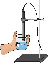
Figure 1

MATERIALS

PROCEDURE

1. Obtain and wear goggles.

2. Add 70 mL of distilled water to a clean 100 mL beaker. Obtain a dropper bottle that contains 1.0 M NaCl solution.

3. Set the selector switch on the side of the Conductivity Probe to the 0–2000 µS/cm range. Connect the Conductivity Probe to LabQuest and choose New from the File menu. If you have an older sensor that does not auto-ID, manually set up the sensor.

4. Set up the data-collection mode.

a. On the Meter screen, tap Mode. Change the mode to Events with Entry.

b. Enter the Name (Volume) and Units (drops). Select OK.

5. Before adding any drops of solution:

a. Start data collection.

b. Carefully raise the beaker and its contents up around the Conductivity Probe until the hole near the probe end is completely submerged in the solution being tested. Important: Since the two electrodes are positioned on either side of the hole, this part of the probe must be completely submerged.

c. Before you have added any drops of NaCl solution, tap Keep. Enter 0, the volume (in drops) and then select OK to save this data pair for this experiment.

d. Lower the beaker away from the probe.

6. You are now ready to begin adding salt solution.

a. Add 1 drop of NaCl solution to the distilled water. Stir to ensure thorough mixing.

b. Carefully raise the beaker and its contents up around the Conductivity Probe until the hole near the probe end is completely submerged in the solution being tested.

c. Briefly swirl the beaker contents. Monitor the conductivity of the solution for about 5 seconds.

d. When the conductivity readings stabilize, tap Keep. Enter 1 as the volume in drops and then select OK. The conductivity and volume values have now been saved for the second trial.

e. Lower the beaker away from the probe.

7. Repeat the Step 6 procedure, entering 2 this time.

8. Continue this procedure, adding 1-drop portions of NaCl solution, measuring conductivity, and entering the total number of drops added—until a total of 8 drops has been added.

9. Stop data collection.

10. To analyze the relationship between conductivity and volume, use this method to calculate the linear-regression statistics for your data. Then plot the linear regression curve on your graph.

a. Choose Curve Fit from the Analyze menu.

b. Select Linear for the Fit Equation. Note: Since increasing the volume (drops) of NaCl increases the concentration of NaCl in the solution, the graph actually represents the relationship between conductivity and concentration. The linear-regression statistics for these two lists are displayed for the equation in the form

y=mx+b

where y is conductivity, x is volume, m is the slope, and b is the y-intercept.

c. Record the value for the slope, m, in your data table.

d. Select OK.

11. Store the data from the first run by tapping the File Cabinet icon.

12. Repeat Steps 5–11, this time using 1.0 M AlCl₃ solution in place of 1.0 M NaCl solution.

13. Repeat Steps 5–10, this time using 1.0 M CaCl₂ solution. Important: Do not store this run as you did in the first two runs—proceed directly to Step 14 after you complete Step 10.

14. To view a graph of concentration vs. volume showing all three data runs, tap Run 3 and select All Runs. All three runs will now be displayed on the same graph axes.

15. (optional) Print a copy of the graph displayed in Step 14. Label each run as “1.0 M NaCl,”
“1.0 M AlCl₃,” or “1.0 M CaCl₂”.

Processing the data

1. Describe the appearance of each of the three curves on your graph in Step 14.

2. Describe the change in conductivity as the concentration of the NaCl solution was increased by the addition of NaCl drops. What kind of mathematical relationship does there appear to be between conductivity and concentration?

3. Write a chemical equation for the dissociation of NaCl, AlCl₃, and CaCl₂ in water.

4. Which graph had the largest slope value? The smallest? Since all solutions had the same original concentration (1.0 M), what accounts for the difference in the slope of the three plots? Explain.

DATA TABLE